Generating Mass Assembly Histories in Diffhalos

In Diffhalos we use DiffmahNet in order to assign MAHs to the (sub)halo populations in the lightcones. DiffmahNet is a population-level model of the Diffmah model for predicting mass assembly histories (MAHs) of individual halos. Once the halos are generated by sampling from the halo and subhalo mass function for hosts and subhalos, respectively, DiffmahNet pastes a MAH onto each (sub)halo in the lightcone, conditioned on mass its \(M_{\rm obs} \equiv M_{\rm halo} (t_{\rm obs})\) at the time of observation \(t_{\rm obs}\).

import matplotlib.pyplot as plt
from matplotlib.lines import Line2D
import matplotlib.patches as mpatches

plt.rc("text", usetex=True)
plt.rc("font", family="serif", size=18)
plt.rcParams.update({'xtick.direction': 'in', 'ytick.direction': 'in'})

Matplotlib is building the font cache; this may take a moment.

import numpy as np
from jax import random as jran
from jax import numpy as jnp

Halo MAHs

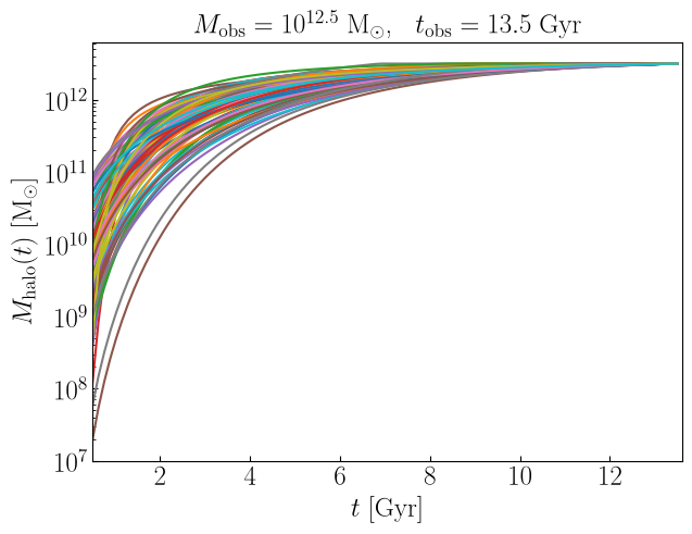
Below, we demonstrate how to produce MAHs for a population of halos, conditioned on a single set of \((t_{\rm obs}, M_{\rm obs})\). In what follows, one must be careful to rescale the MAH parameters from DiffmahNet so that the conditions are exactly satisfied.

from diffhalos.mah.diffmahnet import log_mah_kern
from diffhalos.mah.diffmahnet_utils import mc_mah_cenpop
from diffhalos.mah.utils import rescale_mah_parameters

ran_key = jran.key(0)

n_cens = 100

# conditions for MAH generation
m_obs = np.array([12.5])
t_obs = np.array([13.5])

n_sample = 100
logt0 = np.log10(13.8)

m_vals, t_vals = [
    jnp.repeat(x.flatten(), n_sample)
    for x in np.stack(
        [m_obs, t_obs],
        axis=-1,
    ).T
]

centrals_model_key = "cenflow_v2_0_64bit.eqx"

# compute the MAH parameters
mah_params_uncorr = mc_mah_cenpop(m_vals, t_vals, ran_key, centrals_model_key)

n_t = 100
t_min = 0.5
t_grid = jnp.linspace(t_min, t_vals, n_t).T

# compute observed mass with corrected parameters
logmp_obs_uncorr = log_mah_kern(mah_params_uncorr, t_grid, logt0)

# apply correction to MAH parameters to ensure that the M_halo(t_obs) = M_obs is true for all halos
mah_params = rescale_mah_parameters(mah_params_uncorr, m_vals, logmp_obs_uncorr[:,-1])
logmp_obs = log_mah_kern(mah_params, t_grid, logt0)

fig, ax = plt.subplots(figsize=([7,5]))

_=ax.plot(t_grid.T, 10**logmp_obs.T)

ax.set_xlabel(r"$t\; [{\rm Gyr}]$")
ax.set_ylabel(r"$M_{\rm halo} (t)\; [{\rm M_\odot}]$")

ax.set_yscale('log')

ax.set_xlim([0.5, 13.6])
ax.set_ylim([10**7, 10**12.8])

_=ax.set_title(r"$M_{\rm obs}=10^{12.5}\; {\rm M_\odot}$, \; $t_{\rm obs}=13.5\; {\rm Gyr}$", fontsize=18)

Different choice of \((t_{\rm obs}, M_{\rm obs})\)

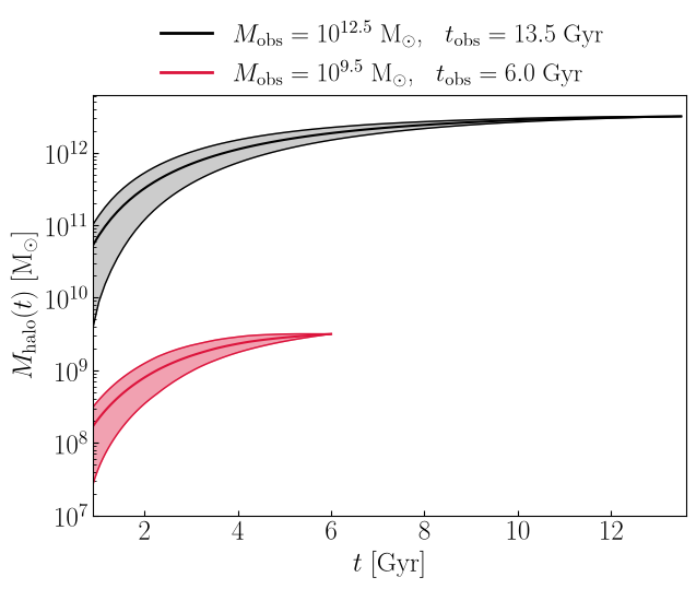
There is nothing special to the conditions we chose above. Below we show that for different sets of \((t_{\rm obs}, M_{\rm obs})\), arbitrarily chosen, the halo population that is produced has a MAH that converges at \(M_{\rm obs}\) at time \(t_{\rm obs}\).

ran_key = jran.key(0)

n_cens = 100

# conditions for MAH generation
m_obs_2 = np.array([9.5])
t_obs_2 = np.array([6.0])

n_sample = 100
logt0 = np.log10(13.8)

m_vals, t_vals = [
    jnp.repeat(x.flatten(), n_sample)
    for x in np.stack(
        [m_obs_2, t_obs_2],
        axis=-1,
    ).T
]

# compute the MAH parameters
mah_params_uncorr = mc_mah_cenpop(m_vals, t_vals, ran_key, centrals_model_key)

n_t = 100
t_min = 0.5
t_grid_2 = jnp.linspace(t_min, t_vals, n_t).T

# compute observed mass with corrected parameters
logmp_obs_uncorr = log_mah_kern(mah_params_uncorr, t_grid_2, logt0)

# apply correction to MAH parameters to ensure that the M_halo(t_obs) = M_obs is true for all halos
mah_params = rescale_mah_parameters(mah_params_uncorr, m_vals, logmp_obs_uncorr[:,-1])
logmp_obs_2 = log_mah_kern(mah_params, t_grid_2, logt0)

from diffhalos.mah.diffmahnet_utils import get_mean_and_std_of_mah

mah_mean, mah_max, mah_min = get_mean_and_std_of_mah(10**logmp_obs)
mah_mean_2, mah_max_2, mah_min_2 = get_mean_and_std_of_mah(10**logmp_obs_2)

fig, ax = plt.subplots(figsize=([7,5]))

plt.plot(t_grid[0], mah_mean, ls='-', color='k')
ax.plot(t_grid[0], mah_max, ls='-', lw=1, color='k')
ax.plot(t_grid[0], mah_min, ls='-', lw=1, color='k')
ax.fill_between(t_grid[0], mah_min, mah_max, color='gray', alpha=0.4)

plt.plot(t_grid_2[0], mah_mean_2, ls='-', color='crimson')
ax.plot(t_grid_2[0], mah_max_2, ls='-', lw=1, color='crimson')
ax.plot(t_grid_2[0], mah_min_2, ls='-', lw=1, color='crimson')
ax.fill_between(t_grid_2[0], mah_min_2, mah_max_2, color='crimson', alpha=0.4)

ax.set_xlabel(r"$t\; [{\rm Gyr}]$")
ax.set_ylabel(r"$M_{\rm halo} (t)\; [{\rm M_\odot}]$")


ax.set_yscale('log')

_=ax.set_xlim([0.9, 13.6])
_=ax.set_ylim([10**7, 10**12.8])

custom_handles = [
    Line2D([0], [0], color='k', lw=2,
           label=r"$M_{\rm obs}=10^{%.1f}\; {\rm M_\odot}$, \; $t_{\rm obs}=%.1f\; {\rm Gyr}$"%(m_obs[0],t_obs[0])),
    Line2D([0], [0], color='crimson', lw=2, ls='-',
           label=r"$M_{\rm obs}=10^{%.1f}\; {\rm M_\odot}$, \; $t_{\rm obs}=%.1f\; {\rm Gyr}$"%(m_obs_2[0],t_obs_2[0])),
]

_=ax.legend(handles=custom_handles, bbox_to_anchor=(0.9, 1.23), frameon=False, ncols=1, fontsize=17)

Generating MAH lightcones

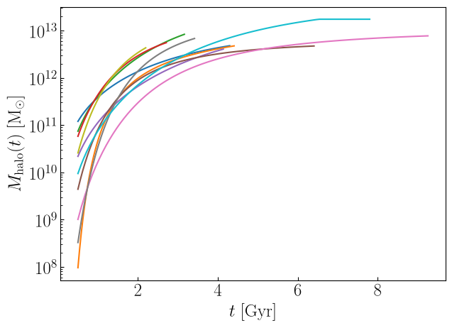
Below we show that the lightcone outputs by default include the MAH of each (sub)halo. In particular, each halo in the generated lightcone is assigned a set of MAH parameters, which can then be used to produce the mass assembly history of each halo using the Diffmah model. Below we plot some of the generated MAHs, chosen randomly for a few halos, for demonstration purposes.

from diffhalos.lightcone_generators import mc_lc

ran_key = jran.key(0)

lgmp_min = 12.5
lgmsub_min = lgmp_min - 0.01
z_min, z_max = 0.4, 3.5
sky_area_degsq = 10.0

args = (ran_key, lgmp_min, lgmsub_min, z_min, z_max, sky_area_degsq)

halopop_mc = mc_lc(*args)

n_t = 100
t_min = 0.5
t_grid = jnp.linspace(t_min, halopop_mc.t_obs, n_t).T

logmp_obs_mah = log_mah_kern(halopop_mc.mah_params, t_grid, halopop_mc.logt0)

import random

fig, ax = plt.subplots(figsize=([7,5]))

indx = np.asarray(random.sample(range(0, len(halopop_mc.t_obs)), 10))

_=ax.plot(t_grid[indx].T, 10**logmp_obs_mah[indx].T)

ax.set_xlabel(r"$t\; [{\rm Gyr}]$")
ax.set_ylabel(r"$M_{\rm halo} (t)\; [{\rm M_\odot}]$")

_=ax.set_yscale('log')