Quickstart

This quickstart guide gives an overview of the core features of Diffhalos, and demonstrates how to use the primary functions of the library.

Monte carlo lightcone

In this mode, the generated lightcone returns halos where each distinct halo has its own mass and redshift. Below we generate a Monte Carlo realization of the lightcone, including host halos and subhalos over a specified range of redshift, and within a given sky area.

from diffhalos.lightcone_generators import mc_lc

from jax import random as jran

ran_key = jran.key(0)

lgmp_min = 12.5
lgmsub_min = lgmp_min - 0.01
z_min, z_max = 0.4, 3.5
sky_area_degsq = 10.0

args = (ran_key, lgmp_min, lgmsub_min, z_min, z_max, sky_area_degsq)

halopop_mc = mc_lc(*args)
print(halopop_mc._fields)

('z_obs', 't_obs', 'logmp_obs', 'mah_params', 'logmp0', 'logt0', 'cen_weight', 'central', 'sat_weight', 'nsub_per_host', 'logmu_obs', 'halo_indx', 'halo_weight')

Mass-function weighting

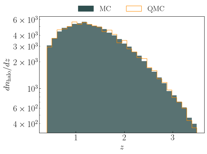
In the weighted version of the generator, every halo and subhalo in the returned lightcone has a weight that encodes the multiplicity of the halo. For any input choice of the number of returned halos, the weights are determined according to the halo and subhalo mass functions. For large enough halo populations, the two versions of the lightcone agree almost perfectly, as demonstrated below where we plot the redshift distributions from the Monte-Carlo (MC) and quasi-Monte Carlo (QMC, i.e. weighted) generators.

import matplotlib.pyplot as plt
from matplotlib.lines import Line2D
import matplotlib.patches as mpatches

plt.rc("text", usetex=True)
plt.rc("font", family="serif", size=20)
plt.rcParams.update({'xtick.direction': 'in', 'ytick.direction': 'in'})

from diffhalos import weighted_lc

ran_key = jran.key(0)

n_host_halos = 70_000
z_min, z_max = 0.4, 3.5
lgmp_min, lgmp_max = 12.5, 15.5
sky_area_degsq = 10.0

args = (ran_key, n_host_halos, z_min, z_max, lgmp_min, lgmp_max, sky_area_degsq)
halopop_qmc = weighted_lc(*args)
print(halopop_qmc._fields)

('z_obs', 't_obs', 'logmp_obs', 'mah_params', 'logmp0', 'logt0', 'cen_weight', 'central', 'sat_weight', 'nsub_per_host', 'logmu_obs', 'halo_indx', 'halo_weight')

fig, ax = plt.subplots(figsize=([7,5]))

plt.hist(halopop_mc.z_obs, bins=30, color='darkslategray', alpha=0.8)
plt.hist(halopop_qmc.z_obs, weights=halopop_qmc.halo_weight, bins=30, color='darkorange', histtype='step')

plt.xlabel(r'$z$')
plt.ylabel(r'$dn_{\rm halo} / dz$')

plt.yscale('log')

custom_handles = [
    mpatches.Patch(edgecolor="darkslategray", lw=1, color='darkslategray', label=r"${\rm MC}$"),
    mpatches.Patch(edgecolor="darkorange", fill=False, lw=1, color='darkorange', label=r"${\rm QMC}$"),
]

_=ax.legend(handles=custom_handles, bbox_to_anchor=(0.8, 1.15), frameon=False, ncols=2, fontsize=18)

/tmp/ipykernel_2465/805277387.py:12: UserWarning: Setting the 'color' property will override the edgecolor or facecolor properties.
  mpatches.Patch(edgecolor="darkslategray", lw=1, color='darkslategray', label=r"${\rm MC}$"),
/tmp/ipykernel_2465/805277387.py:13: UserWarning: Setting the 'color' property will override the edgecolor or facecolor properties.
  mpatches.Patch(edgecolor="darkorange", fill=False, lw=1, color='darkorange', label=r"${\rm QMC}$"),

Compare host and subhalo populations separately by identifying them in the lightcone output

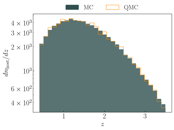
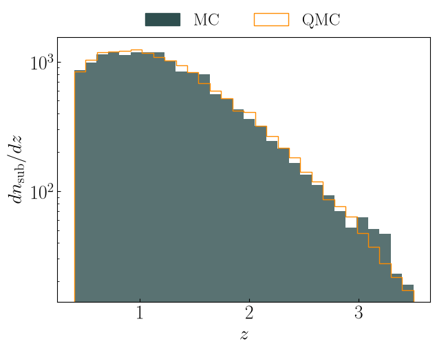
So far we have plotted halos and subhalos together. Below we demonstrate how one can distinguish between the two populations in the generated lightcones and use them separately. As we show in the plots, for each populations separately, MC and QMC are still in great agreement with each other.

import numpy as np

is_cen_mc = np.where(halopop_mc.central==1)[0]
is_sat_mc = np.where(halopop_mc.central==0)[0]
is_cen_qmc = np.where(halopop_qmc.central==1)[0]
is_sat_qmc = np.where(halopop_qmc.central==0)[0]

fig, ax = plt.subplots(figsize=([7,5]))

plt.hist(halopop_mc.z_obs[is_cen_mc], bins=30, color='darkslategray', alpha=0.8)
plt.hist(halopop_qmc.z_obs[is_cen_mc], weights=halopop_qmc.halo_weight[is_cen_mc], bins=30, color='darkorange', histtype='step')

plt.xlabel(r'$z$')
plt.ylabel(r'$dn_{\rm host} / dz$')

plt.yscale('log')

custom_handles = [
    mpatches.Patch(edgecolor="darkslategray", lw=1, color='darkslategray', label=r"${\rm MC}$"),
    mpatches.Patch(edgecolor="darkorange", fill=False, lw=1, color='darkorange', label=r"${\rm QMC}$"),
]

_=ax.legend(handles=custom_handles, bbox_to_anchor=(0.8, 1.15), frameon=False, ncols=2, fontsize=18)

/tmp/ipykernel_2465/3984482598.py:12: UserWarning: Setting the 'color' property will override the edgecolor or facecolor properties.
  mpatches.Patch(edgecolor="darkslategray", lw=1, color='darkslategray', label=r"${\rm MC}$"),
/tmp/ipykernel_2465/3984482598.py:13: UserWarning: Setting the 'color' property will override the edgecolor or facecolor properties.
  mpatches.Patch(edgecolor="darkorange", fill=False, lw=1, color='darkorange', label=r"${\rm QMC}$"),

fig, ax = plt.subplots(figsize=([7,5]))

plt.hist(halopop_mc.z_obs[is_sat_mc], bins=30, color='darkslategray', alpha=0.8)
plt.hist(halopop_qmc.z_obs[is_sat_qmc], weights=halopop_qmc.halo_weight[is_sat_qmc], bins=30, color='darkorange', histtype='step')

plt.xlabel(r'$z$')
plt.ylabel(r'$dn_{\rm sub} / dz$')

plt.yscale('log')

custom_handles = [
    mpatches.Patch(edgecolor="darkslategray", lw=1, color='darkslategray', label=r"${\rm MC}$"),
    mpatches.Patch(edgecolor="darkorange", fill=False, lw=1, color='darkorange', label=r"${\rm QMC}$"),
]

_=ax.legend(handles=custom_handles, bbox_to_anchor=(0.8, 1.15), frameon=False, ncols=2, fontsize=18)

/tmp/ipykernel_2465/1531268380.py:12: UserWarning: Setting the 'color' property will override the edgecolor or facecolor properties.
  mpatches.Patch(edgecolor="darkslategray", lw=1, color='darkslategray', label=r"${\rm MC}$"),
/tmp/ipykernel_2465/1531268380.py:13: UserWarning: Setting the 'color' property will override the edgecolor or facecolor properties.
  mpatches.Patch(edgecolor="darkorange", fill=False, lw=1, color='darkorange', label=r"${\rm QMC}$"),

Host halo generator compared to exact theoretical prediction

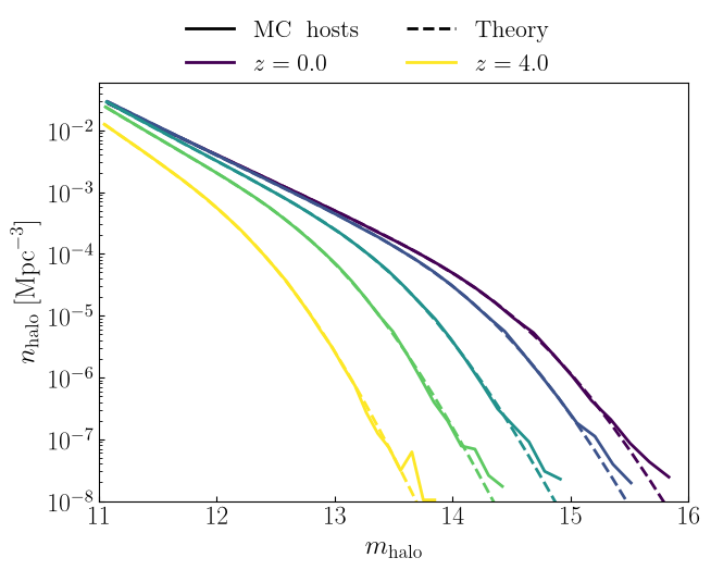
If we produce a halo population, from a lightcone generation, at a specific redshift and bin the halos in mass to infer their distribution, the result must agree with the exact theory prediction from the underlying halo mass function (HMF) model. We show that this is true below, at various redshifts. Note that we define \(m_{\rm halo} \equiv \log_{10} M_{\rm halo}\).

from diffhalos.hmf.mc_hosts import mc_host_halos_singlez
from diffhalos.hmf.hmf_model import _compute_nhalos_tot, DEFAULT_HMF_PARAMS, predict_diff_hmf

ran_key = jran.key(0)

lgmp_min = 11.0
lgmsub_min = lgmp_min - 0.01
Lbox = 1000.0
volume_com_mpc = Lbox**3

z_grid = [0.01, 0.5, 1.5, 2.5, 4.0]

bins = 30

import matplotlib.cm as cm
colors = cm.viridis(np.linspace(0,1,len(z_grid)))

tick_fontsize = 17
label_fontsize = 18
legend_fontsize = 16

fig, ax = plt.subplots(figsize=([7,5]))

for iz, zi in enumerate(z_grid):

    z_min = zi-0.005
    z_max = zi+0.005

    args = (ran_key, lgmp_min, lgmsub_min, z_min, z_max, sky_area_degsq)

    # MC host halos
    mc_logmhalo = mc_host_halos_singlez(ran_key, lgmp_min, zi, volume_com_mpc)

    # bin generated host masses
    hist_data = np.histogram(mc_logmhalo, bins=bins, density=False)

    dlogm_bin_edges = hist_data[1]
    dlogm_bins = 0.5 * (dlogm_bin_edges[1:] + dlogm_bin_edges[:-1])

    n_halo = mc_logmhalo.size
    n_tot = _compute_nhalos_tot(
        DEFAULT_HMF_PARAMS,
        lgmp_min,
        zi,
        volume_com_mpc,
    )

    # normalize counts
    dnhalo_bins = hist_data[0] / np.diff(dlogm_bin_edges) / volume_com_mpc
    dnhalo_bins *= n_tot / n_halo

    # theory prediction
    diff_hmf = predict_diff_hmf(DEFAULT_HMF_PARAMS, dlogm_bins, zi)

    ax.plot(dlogm_bins, dnhalo_bins, color=colors[iz], lw=2)
    ax.plot(dlogm_bins, 10**diff_hmf, color=colors[iz], ls='--', lw=2)

ax.tick_params(axis='both', which='major', labelsize=tick_fontsize)
ax.tick_params(axis='both', which='minor', labelsize=tick_fontsize)

ax.set_xlabel(r"$m_{\rm halo}$", fontsize=label_fontsize)
ax.set_ylabel(r"$n_{\rm halo}\; [{\rm Mpc}^{-3}]$", fontsize=label_fontsize)

ax.set_yscale('log')

ax.set_xlim([11.0, 16.0])
ax.set_ylim([1e-8, 6e-2])

custom_handles = [
    Line2D([0], [0], color='k', lw=2, label=r"{\rm MC\; hosts}"),
    Line2D([0], [0], color=colors[0], lw=2, label=r"$z=%.1f$"%z_grid[0]),
    Line2D([0], [0], color='k', lw=2, ls='--', label=r"{\rm Theory}"),
    Line2D([0], [0], color=colors[-1], lw=2, label=r"$z=%.1f$"%z_grid[-1]),
]

_=ax.legend(handles=custom_handles, bbox_to_anchor=(0.8, 1.2), frameon=False, ncols=2, fontsize=legend_fontsize)

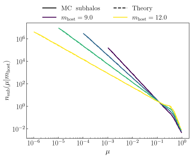
Subhalo generator compared to exact theoretical prediction

Similarly to halos, if we generate a subhalo population, conditioned on the host mass at a given redshift, and bin in \(\mu \equiv M_{\rm sub}/M_{\rm host}\) to infer their distribution, the result must agree with the exact theory prediction from the conditional subhalo mass function (CSHMF) model. We show that this is the case below, for various host halo masses. Since we have shown already that the MC and QMC subhalo lightcones agree with each other, below we utilize the weighted lightcone generator to speed up the computations and to reduce the memory footprint.

from diffhalos.lightcone_generators import weighted_lc_subhalos
from diffhalos.lightcone_generators.utils import generate_mock_cenpop
from diffhalos.ccshmf.ccshmf_model import predict_diff_cshmf, DEFAULT_CCSHMF_PARAMS

lgmhost_arr = np.linspace(9.0, 12.0, 4)
lgmsub_min = 6.0

z_min = 0.99
z_max = 1.01

import matplotlib.cm as cm
colors = cm.viridis(np.linspace(0,1,len(lgmhost_arr)))

bins = 30
n_mu_per_host = 500

fig, ax = plt.subplots(figsize=([7,5]))

for im, mi in enumerate(lgmhost_arr):

    logmp_min = mi-0.01
    logmp_max = mi+0.01

    cenpop = generate_mock_cenpop(z_min, z_max, logmp_min, logmp_max, n_cens=1)

    subpop = weighted_lc_subhalos(ran_key, cenpop, lgmsub_min, n_mu_per_host=n_mu_per_host)

    # bin in mu
    hist_data = np.histogram(subpop.logmu_obs, weights=subpop.sat_weight, bins=bins, density=False)
    dlogmu_bin_edges = hist_data[1]
    dlogmu_bins = 0.5 * (dlogmu_bin_edges[1:] + dlogmu_bin_edges[:-1])

    # normalize counts
    dnsub_bins = hist_data[0] / np.diff(dlogmu_bin_edges)

    # theory prediction
    logmu_arr = np.linspace(subpop.logmu_obs.min(), subpop.logmu_obs.max(), 200)
    cshmf_theory = predict_diff_cshmf(DEFAULT_CCSHMF_PARAMS, mi, logmu_arr)

    ax.plot(10**dlogmu_bins, dnsub_bins, color=colors[im], lw=2)
    ax.plot(10**logmu_arr, 10**cshmf_theory, color=colors[im], ls='--', lw=2)

ax.tick_params(axis='both', which='major', labelsize=tick_fontsize)
ax.tick_params(axis='both', which='minor', labelsize=tick_fontsize)

ax.set_xlabel(r"$\mu$", fontsize=label_fontsize)
ax.set_ylabel(r"$n_{\rm sub} (\mu | m_{\rm host})$", fontsize=label_fontsize)

ax.set_xscale('log')
ax.set_yscale('log')

custom_handles = [
    Line2D([0], [0], color='k', lw=2, label=r"{\rm MC\; subhalos}"),
    Line2D([0], [0], color=colors[0], lw=2, label=r"$m_{\rm host}=%.1f$"%lgmhost_arr[0]),
    Line2D([0], [0], color='k', lw=2, ls='--', label=r"{\rm Theory}"),
    Line2D([0], [0], color=colors[-1], lw=2, label=r"$m_{\rm host}=%.1f$"%lgmhost_arr[-1]),
]

_=ax.legend(handles=custom_handles, bbox_to_anchor=(0.9, 1.2), frameon=False, ncols=2, fontsize=legend_fontsize)