Differences between Monte Carlo and quasi-Monte Carlo

This notebook presents the main differences between the two modes of lightcone generation with Diffhalos: the Monte Carlo (MC) and the quasi-Monte Carlo (QMC), also called weighted, lightcone. While in the MC version we randomly distribute each halo in redshift \(z\) and mass \(M_{\rm halo}\) (using the halo mass function; HMF), in the case of QMC we contruct a uniform grid of \((z,m_{\rm halo})\), where \(m_{\rm halo} \equiv \log_{10} M_{\rm halo}\). Then, in the QMC lightcone each point is assigned a weight that represents the expected abundance of halos, according to an underlying HMF model.

For subhalos the difference between the two versions of the lightcone is analogous to the host halo generation above. In the MC lightcone, for each individual (host) halo, generated according to the above, we draw samples from the conditional subhalo mass fucntion (CSHMF; as a function of the parameter \(\mu \equiv M_{\rm sub}/M_{\rm host}\)), and thus populate each of them with the subhalos they host. In the QMC version, at each point in the preconstructed grid of redshift and mass for hosts from above, we first create a grid of \(\mu\) values (typically \(3-5\)) between a minimum and a maximum, and then we assign a weight to each point that represents the abundance of subhalos.

import matplotlib.pyplot as plt
from matplotlib.lines import Line2D
import matplotlib.patches as mpatches

plt.rc("text", usetex=True)
plt.rc("font", family="serif", size=17)
plt.rcParams.update({'xtick.direction': 'in', 'ytick.direction': 'in'})

Visualizing a Monte Carlo lightcone

In the cells below, we create a MC lightcone and we visualize how the points populate the \(z-m_{\rm halo}\) plane.

from diffhalos.lightcone_generators.mc_lightcone_halos import mc_lc_halos

from jax import random as jran

ran_key = jran.key(0)

lgmp_min = 12.5
lgmsub_min = lgmp_min - 0.01
z_min, z_max = 0.1, 4.0
sky_area_degsq = 10.0

args = (ran_key, lgmp_min, z_min, z_max, sky_area_degsq)

halopop_mc = mc_lc_halos(*args)

plt.figure(figsize=([6,5]))

plt.scatter(halopop_mc.z_obs, 10**halopop_mc.logmp_obs, s=1, color='cadetblue')

plt.yscale('log')

plt.xlabel(r"$z$")
_=plt.ylabel(r"$M_{\rm halo}\; [{\rm M_\odot}]$")

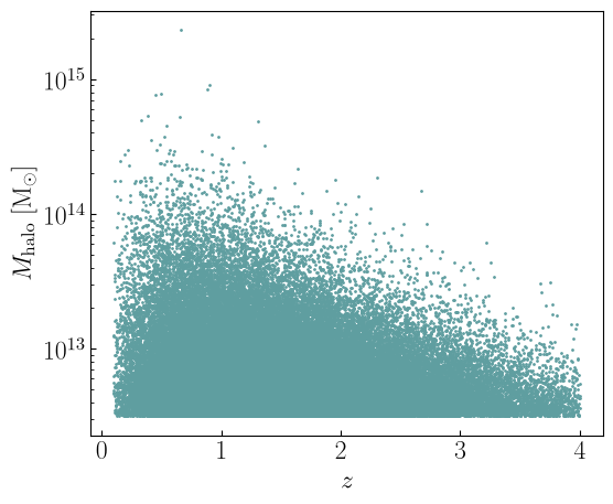
The general trends we observe are as expected. From high to low redshift the maximum halo mass increases, as more massive halos form over cosmic time. Also, the abundance of low-mass halos is larger per redshift slice due to the shape of the HMF which increases as a steep power-law in \(\Lambda\)CDM cosmologies at the low-mass regime.

The total number of halos in the generated lightcone is not predetermined, but rather computed according to the input parameters. In particular, between redshifts \(z_{\min} < z < z_{\max}\) and given a range of halo mass \(M_{\min} < M_{\rm halo} < M_{\max}\), we first compute a mean number of halos using the cumulative HMF \(n_{\rm halo}(>M_{\rm halo},z)\). Once this is done for the whole lightcone, we generate Poisson realizations of the number of halos, so that each generated lightcone is slightly different.

halopop_mc.z_obs.size

79096

Visualizing a quasi-Monte Carlo lightcone

We now create a visualization of a weighted halo lightcone.

from diffhalos.lightcone_generators.mc_lightcone_halos import weighted_lc_halos

ran_key = jran.key(0)

n_host_halos = 10000
z_min, z_max = 0.1, 4.0
lgmp_min, lgmp_max = 12.5, 15.5
sky_area_degsq = 10.0

args = (ran_key, n_host_halos, z_min, z_max, lgmp_min, lgmp_max, sky_area_degsq)
halopop_qmc = weighted_lc_halos(*args)

import numpy as np

plt.figure(figsize=([6,5]))

scatter = plt.scatter(halopop_qmc.z_obs, 10**halopop_qmc.logmp_obs, s=1, c=np.log10(halopop_qmc.cen_weight), cmap='viridis')

cbar = plt.colorbar(scatter)
cbar.set_label(r'$\log_{10} n_{\rm halo}$')

plt.yscale('log')

plt.xlabel(r"$z$")
_=plt.ylabel(r"$M_{\rm halo}\; [{\rm M_\odot}]$")

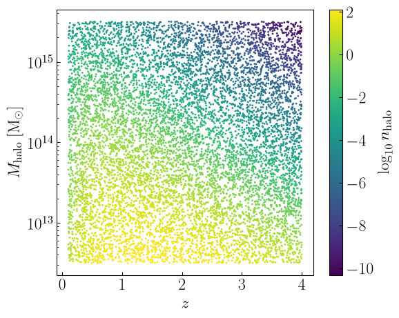
As we see, the points are now uniformly distributed in redshist and halo mass. Additionally, we see a general trend where the weights (the plot is color-coded based on the base-10 log of the halo weights, in this case the differential HMF model prediction) increase from top-right to bottom-left, as lower-mass, lower-redshift halos are generally more abundant.

Using the weighted lightcones

When using the QMC lightcone outputs for any kind of computation involving halo statistics, attention is needed to ensure that the weights are utilized properly. Since each point in the generated grid is simply the result of uniformly distributing halos in redshift and mass, the weights encode all the necessary information of the halo abundance when computing statistical quantities.

For example, to plot the distribution of the generated halos as a function of redshift, we need to use the property cen_weight in the output to properly weight the histogram. Below we demonstrate this.

plt.figure(figsize=([5,4]))

_=plt.hist(halopop_qmc.z_obs, weights=halopop_qmc.cen_weight, bins=20, color='darkred', alpha=0.6)

plt.yscale('log')

plt.xlabel(r"$z$")
_=plt.ylabel(r"$N_{\rm halos}$")

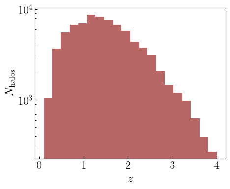
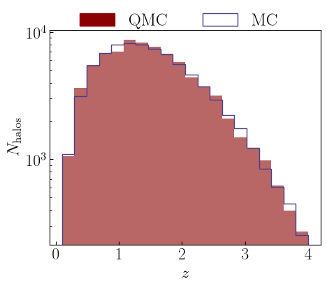
When using the MC lightcone, there is no need to weight since the generated halos in it already have the proper abundance. In addition, in the limit where the number of generated halos is large enough, the MC and QMC lightcones should look almost identical. Below we show that this is roughly the case, even for the relatively low number of halos in the lightcones in this notebook. For a more careful comparison, see diffhalos_quickstart.ipynb.

fig, ax = plt.subplots(figsize=([5,4]))

_=plt.hist(halopop_qmc.z_obs, weights=halopop_qmc.cen_weight, bins=20, color='darkred', alpha=0.6)
_=plt.hist(halopop_mc.z_obs, bins=20, color='darkslateblue', histtype='step')

plt.yscale('log')

plt.xlabel(r"$z$")
plt.ylabel(r"$N_{\rm halos}$")

custom_handles = [
    mpatches.Patch(color="darkred", lw=1, label=r"${\rm QMC}$"),
    mpatches.Patch(color="darkslateblue", fill=False, lw=1, label=r"${\rm MC}$"),
]

_=ax.legend(handles=custom_handles, bbox_to_anchor=(0.9, 1.15), frameon=False, ncols=2, fontsize=18)